This lesson begins our video series on neural networks in artificial intelligence. Neural networks come in numerous varieties, and the perceptron is considered one of the most basic. Frank Rosenblatt developed the algorithm in 1957. The single-layer version given here has limited applicability to practical problems. However, it is a building block for more sophisticated and usable systems.

As token applications, we mention the use of the perceptron for analyzing stocks and medical images in the video. In truth, a single-layer perceptron would not perform very well for these. On the other hand, with multiple perceptrons and higher-dimensional data, we reasonably expect some useful predictions or diagnoses.

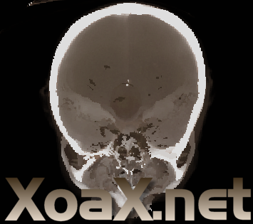
In medical imaging, for example, a computer program could extract features from multiple modalities automatically collect the data as a feature set and apply a trained neural network to assist physicians in making a diagnosis. What is particularly appealing about that is that the computer is less prone to error for rote tasks. However, a neural network is not capable of understanding at a level to make a proper diagnosis, as a physician would. The image above is from a volume-rendering program that I wrote, a subject we will go over when we cover graphics and image processing.

Let's return to our stock analysis example. In the video, I mentioned that we could predict whether a stock is a buy or sell based on a few factors. For example, we might take a set of stocks that gained or lost 5% last month and call them a buy or sell. Looking at the month before that, we could extract our prediction features as the return and percent change in volume from the previous month. This technique is a form of technical analysis. Looking at a set of stocks, assume that we get a table of values that looks like this:

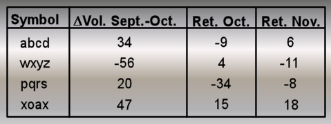
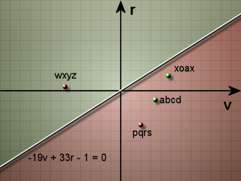
In the first column, we define a fictitious symbol for four stocks. The first two columns are the parameters that we will use for prediction. The third column defines whether the stock is a buy or sell. In this case, the first and fourth stocks are buys and the other two are sells.

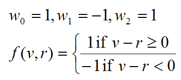
Here is the classification function:

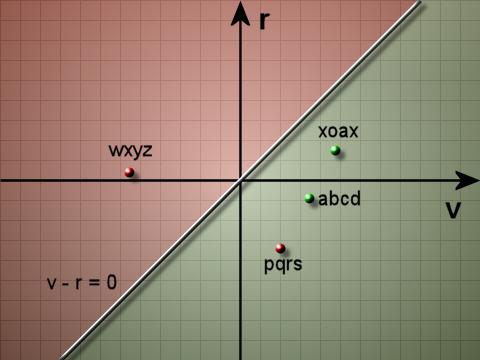
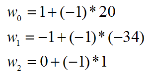
From the image, it is clear that "pqrs" is misclassified. So, we subtract its value and the bias from the weights. Although the numbers were given as percentages, we are writing them here as whole numbers because the issue of scale is irrelevant to the algorithm.

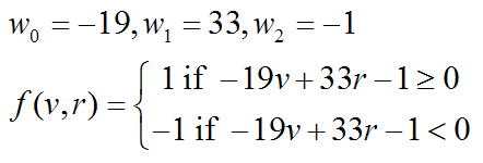
After making the adjustment to the weights, we get the classification function below. Now, "pqrs" is correctly classified, but the other stocks are misclassified. It is not clear that anything has been gained, but it can be proven that the algorithm correctly converges.

This is the classification function for the graph above.

Continually applying the adjustments for misclassified points will get us to the correct classifier. You should try writing the code and testing it to verify convergence.